Ironically, the best solutions for hard problems often involve taking shots in the dark.
Everyone loves control, but the problem is you can’t do everything at once. You can’t count the grains of sand on a beach, because even with the utmost determination, the grains are constantly being moved to and from the beach as you count. But one person could easily use randomness to sample a variety of places on a beach to calculate about how much sand in a fraction of the time.
A similar issue happens in system optimization when trying to find the “global optima” (the absolute best configuration) of a complex system with many parts. It’s not possible to try every configuration of the system, but if you only change one part of the system at a time, then you can get stuck in a “local optima.”
The Trap of Local Optima
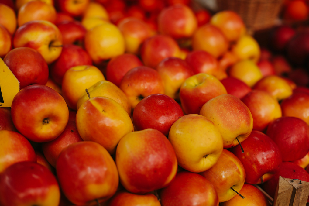
Imagine you’re looking for the largest apple at the grocery store. So you start at one side, and after a few minutes, you find the largest one out of one box. How do you know this is the largest one in all boxes? You don’t. That’s local optima: the best solution to a subset of a problem (e.g., if you’re using only a part of the data). Also, if it takes 2 minutes per box, I’ll be here for half an hour. That’s the trap: you can find the best solution for a small subset quickly, but the absolute best solution takes much longer.
Now, imagine if you just randomly move to a different box every once in a while. Eventually, you’d be looking at an apple variety like Fuji that’s generally bigger to give you a better chance of finding the global optima. But how do you know when to move to the next box and which box to move to? It turns out, an analogy in metallurgy can help us.
Simulated Annealing
Inspired by metallurgy, Simulated Annealing mimics how metals cool and crystallize. At high temperatures, atoms move freely, exploring many arrangements. As the temperature drops, movement slows, and the most stable structure solidifies.
For an optimization algorithm: Early in the process, large random jumps help explore; later, as the algorithm “cools,” randomness decreases, and the solution stabilizes. Mathematically, the chance of accepting a better move is proportional to:
$$ \begin{aligned} &P(\text{accepting better move}) \approx 1 - e^{\frac{\Delta E}{kT}} \\ &\text{where}\\ &\hspace{1em}\Delta E = \text{Amount the result is worsened} \\ &\hspace{1em}T = \text{Temperature} \\ &\hspace{1em}k = \text{A constant relating temperature to energy} \end{aligned} $$As T decreases, the probability of accepting a worse solution and the amount the result can be worsened decrease.
In the apple example, this would be analogous to scanning all the apple types in the store first before focusing on a few promising boxes later. This is an efficient way to use randomness for large datasets.
Monte Carlo Methods
Instead of just searching for an apple, what if you wanted to know the range of apple sizes by variety? Monte Carlo Methods use randomness to approximate a piece of data using random sampling. Instead of looking through all apples one by one, you estimate it by averaging random samples. In modern science, Monte Carlo simulations underpin everything from climate models to financial forecasts. Randomness, repeated often enough, becomes a mirror of reality.
Productive Chaos
Randomness is a tool to find reasonably good solutions to large problems. It can be used to explore a wide range of possibilities, allowing for the discovery of new insights and solutions that might not be found through more straightforward methods. By introducing randomness into optimization algorithms, we can avoid getting stuck in local optima and instead find more globally optimal solutions.